Linear solvers

As a sub-problem for nearly all simulation disciplines, linear systems must be solved. More specifically, the system matrix for process models in SigmaMu can reach O(10000) for models with large scope and/or level of detail.

Note

As SigmaMu formulates most of the model via explicit relationships of properties, the system size is by about two magnitudes lower than in other equation oriented modelling tools, such as gPROMs or Modelica. The explicit formulation includes the entire thermodynamic model formulation and calculation of physical properties.

As an example, a process of 10 packed columns, where each packing is discretised into 10 slices - or 10 tray columns with 10 stages each, and the gas liquid boundary layer of each slice is discretised into 10 reactive elements, an eight-species system yields typically 10 x 10 x 10 x (8 + 2) = 10000 variables.

Typically, the sparsity of the system matrices is around 1 % to 2 %, slightly decreasing with size, as it is rather the number of non-zero elements per row that is constant than the absolute density.

Casadi solver

CasADi features high performant and efficient functionality for solving differential equation systems that come with control problems, and, as a very essential part of SigmaMu, we obtain Jacobian information from the library. Within the SigmaMu solvers, we hence retrieve the system matrices as casadi.DM objects. Though it is possible to solve smaller linear systems, these are not designed to be subject to larger computations.

Scipy solver

The scipy.sparse.linalg module offers spsolve. To utilise this, we first must convert the casadi.DM matrix into a scipy.sparse.csr_matrix, which is made easy by CasADi:

from scipy.sparse import csc_matrix

dm_matrix = DM(...)  # or coming back from a casadi function
...
scipy_matrix = csr_matrix(dm_matrix)

The SciPy module is capable of solving the sparse system of size 10⁴ in about 100 seconds, but not exploiting multiple CPUs in the calculation. One declared target of SigmaMu is to scale its performance with available CPUs.

Pypardiso solver

The Intel oneAPI Math Kernel Library PARDISO solver is wrapped into a python package called PyPardiso. Its spsolve function is compatible to the scipy.sparse.linalg.spsolve version, but exploits available cores.

Performance and comparison

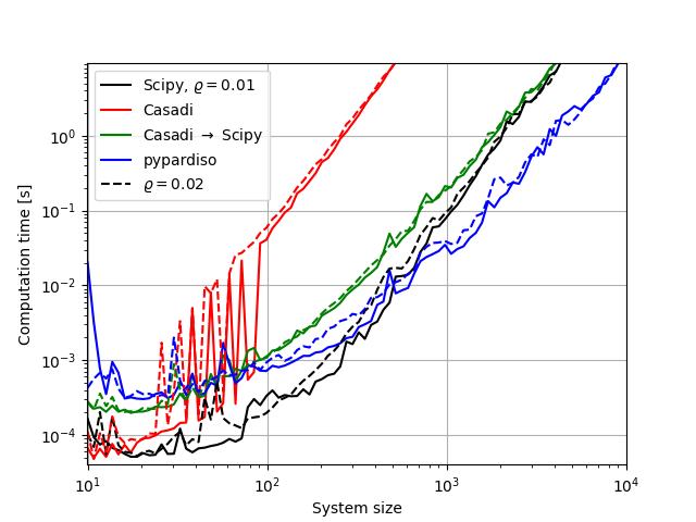
Above figure shows the required runtimes to solve systems of various sizes \(N\) using the above mentioned solvers. We populated a sparse matrix with 1 % or 2 % random valued elements \(a_{ij} \in [0;1]\) and added positive diagonal elements \(a_{ii} > N\) to avoid singularities.

The initial question whether to not bother converting from casadi.DM is answered fast. The performance is by factor 100 below that of SciPy, and systems with sizes larger than some hundred variables would be heavily impacted by this bottle-neck.

All solvers solve, as expected, in cubic time, and whether the density of non-zero elements is 1 % or 2 % has no significant impact. Further, the conversion from CasADi to SciPy has vanishing impact for systems of size greater 1000.

PyPardiso is almost one magnitude faster than SciPy on a PC with 4 CPU cores and 2 threads per core. A system of size 10⁴ can be solved in about 10 seconds.

Warning

However, even for well conditioned systems, PyPardiso sometimes fails to deliver the correct solution and delivers a vector that yields highly non-zero elements in the remaining residual \(b-A\,x\). The same happens even with the sparse SciPy solver, but only with less well conditioned / scaled matrices.

Conclusion

For moderate systems, we could suffice with the standard SciPy solver, but while the model evaluation is of linear to quadratic complexity, the solver will become the bottle-neck eventually. At this point it is advantageous to use PyPardiso and benefit from scalability options by employing multiple cores.

The actual system matrices are somewhat different in structure compared to this test, as they are closer to (while not entire) a block structure. This might have impact on the performance - more likely positive than negative, but will unlikely change the conclusion and performance assessment of the solvers relative to each other.

As a final remark, system sizes of 10⁴ can still be solved comfortably, while things become very slow at 10⁵, given that the solving of one system is only part of an iterative process. If solving such large system became relevant, iterative linear solvers should be considered.

For all solvers, we iteratively transform the system by normalizing rows and columns of the system matrix to mitigate the unavoidable badly scaled variables from our thermodynamic systems. This helps the solvers much to chose feasible pivot elements and yield a valid solution.

Yet, a robust approach is to fall-back on SciPy if PyPardiso gives a wrong solution, and even fall back to NumPy dense matrices if the system size is small enough.